
Chapter 5
Change detection
Change detection compares the state of an area in two different periods and delineates the polygons where the terrain changed according to criteria that you set. It uses Sentinel-2 imagery and mathematical calculations (indices and thresholds); it does not use artificial intelligence. The result is indications that require verification, never a determination about their cause or legality.
There are two entry points: the “Monitoring” tool in the viewer (“Changes” and “Burns” tabs) and the “Change detection” page in the side menu, “Monitoring” group. Both request the analysis from the same engine. Burns are covered in chapter 6.
Requesting an analysis from the viewer
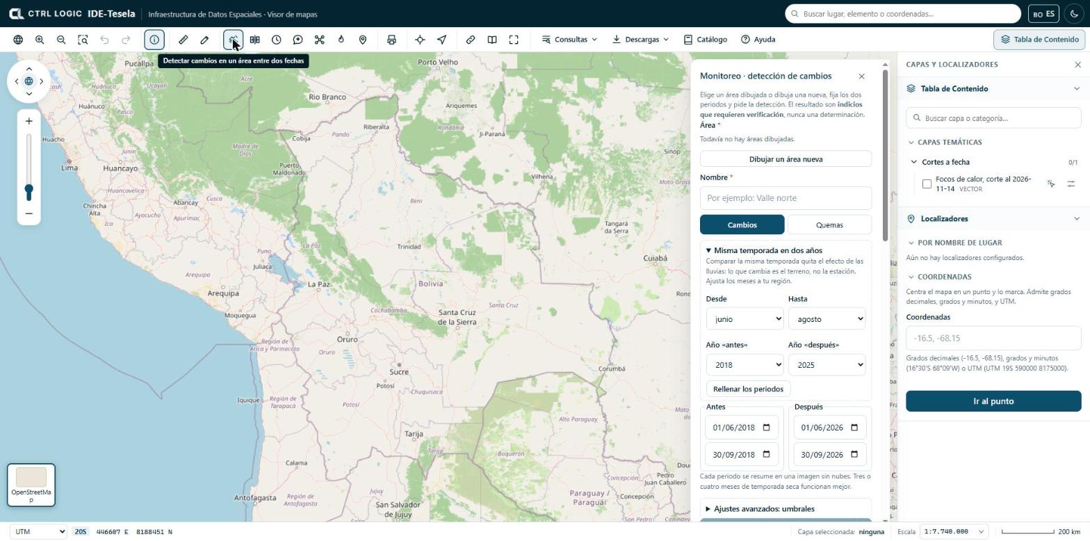
- Click “Monitoring” on the toolbar. The “Monitoring · change detection” panel opens.
- Define the area. You can choose an area you have already drawn, a polygon selected through “Identify → Detect changes here”, or click “Draw a new area”: click on the map for each vertex and double-click to close.
- Enter a name so that you can recognize the analysis later.
- Leave the “Changes” tab active (the “Burns” tab is covered in chapter 6).
- Set the “Before” and “After” periods (see below).
- If necessary, adjust the thresholds under “Advanced settings: thresholds”.
- Click “Detect changes”. The job is queued and takes a few minutes.
Periods and “Same season in two years”
Each period (start and end) is summarized in a single cloud-free image, calculated as the median of the available scenes. Three or four months of dry season work best; with less, there may be no clean image.
Comparing any two dates mixes real change with the effect of the rains. The “Same season in two years” block avoids this: you choose the months (“From” and “To”), the “Year before” and the “Year after”, and click “Fill in the periods”. The initial months are June to August; adjust them to your region. If the season has not started yet in one of the years, the panel asks you to choose an earlier year.
If your institution has more than one imagery provider configured, the “Imagery from” selector appears.
Advanced thresholds
A polygon counts as a change when the “after − before” difference meets all the conditions that are ticked. The initial values are:
| Index | What it measures | Initial condition |
|---|---|---|
| NDVI | Vegetation vigor | Active: drops by at least 0.2 |
| BSI | Bare soil | Inactive: rises by at least 0.1 |
| NBR | Burning and vegetation moisture | Inactive: drops by at least 0.15 |
| NDWI | Surface water | Inactive: rises by at least 0.15 |
Where there is vegetation, a drop in NDVI is enough. In areas without vegetation (highlands, desert) it is better to use bare soil (BSI rises) or NBR (drops). The “Minimum patch (ha)” is also set, which discards smaller polygons; the initial value is 0.5 ha.
Following your analyses
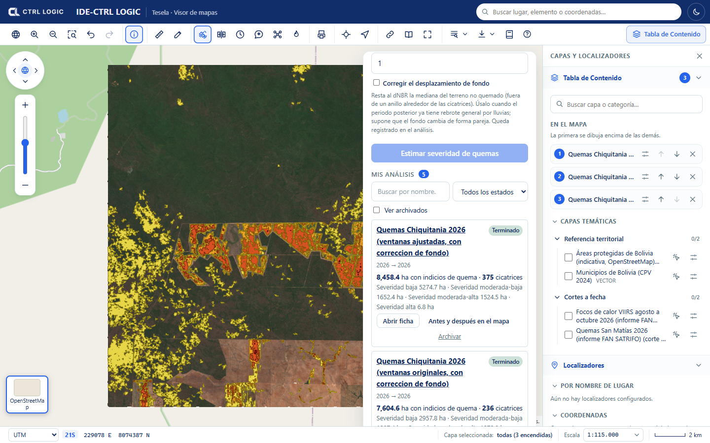
Below the form, “My analyses” appears. Each card shows the status (Queued, Processing, Completed, Failed or Cancelled), the number of polygons and the hectares with indications, or “No changes” when no polygon met the rule. You can search by name and filter by status. A failed analysis can be retried (“Retry”) and a queued one can be cancelled (“Cancel”).
The analysis sheet
“Open sheet” shows the whole analysis in a window:
- At the top, the “before” period against the “after” period, with a swipe handle that you drag to compare, and the label “indications that require verification”.
- Visualization tabs to see the same scene in different ways (see below) and an “Indications” checkbox that draws the polygons on top.
- Figures: number of polygons, hectares with indications and hectares analyzed, broken down by type of change.
- “Polygons by area”: a table with the number, type, hectares and NDVI variation of each zone.
- “Traceability”: periods, rule used, minimum patch, creation date, duration and source of the imagery.
The types of change that can be assigned are “Vegetation loss”, “Exposed soil”, “New water” and “Unclassified”. They are descriptive categories of the type of alteration, not assessments of its origin.
From the sheet you can click:
- “Before and after on the map”: opens the viewer’s comparison tool with the two dates already loaded (chapter 8).
- “Only indications on the map”: switches on only the polygons.
- “Evidence sheet (PDF)”: generates a PDF with the images, the table of zones, how the result was obtained and the statement “These results require verification”.
Scenes by period
For the “before” and the “after” period, each analysis publishes several scenes that help interpret what was detected:
| Scene | What it is for |
|---|---|
| Natural color | What the eye would see |
| False color | Highlights healthy vegetation in bright red |
| SWIR | Shows soil and moisture; bare soil stands out |
| NDVI | Vegetation vigor |
| NDWI | Surface water |
| NDSI | Snow and ice |
An urban false color (built-up surfaces and disturbed soil) is also generated. If an analysis ends with “No changes”, the scenes are still available: compare them by eye and, if you see differences, repeat the analysis with other thresholds.
Archiving and deleting
- Archive removes the analysis from the list without deleting it. It stays intact and can be seen by ticking “Show archived”; “Return to the list” brings it back to “My analyses”.
- Delete removes the analysis permanently, with its scenes and its polygons. The system asks “Delete permanently, with its scenes and polygons?”; it is deleted only if you confirm with “Yes, delete”. This cannot be undone. They are available only when the analysis is no longer in progress.
If you only want to tidy your list, use “Archive”. “Delete” is final.
Limits
- Resolution: Sentinel-2 pixels are 10 to 20 m. It detects changes down to fractions of a hectare; it does not see very small interventions or what happens under cover.
- Clouds: in tropical areas or in the rainy season there may be no clean image for weeks. This is mitigated with longer periods or the same season in two years. Radar (Sentinel-1) is planned but not yet available.
- Thresholds: how much an index must vary to count as a change depends on the terrain. Without local calibration, the result may overestimate or underestimate.
- A polygon is an alteration detected between two images: it does not indicate the cause or whether it is legal. It always requires verification.
Summary
- Draw an area, name it, set the “before” and “after” periods (ideally the same season) and click “Detect changes”.
- The initial rule is a drop in NDVI of at least 0.2 with a minimum patch of 0.5 ha; it is adjusted under “Advanced settings”.
- The analysis sheet brings together the comparison, the polygons, the traceability and the scenes by period.
- “Before and after on the map” opens the comparison tool; “Archive” hides; “Delete” removes permanently and asks for confirmation.
- Every result is an indication that requires verification.